ScanNav Documentation
Charts Workshop
ScanNav opens by default in the mode it was on last usage,
and in Navigation mode if it is the first usage.
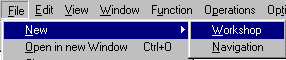
To open a window in Workshop mode when you were previously
in Navigation mode, use the “New” entry of the “File” menu.
Building
Charts:
The first thing to do is to have images to work with.
To do so, you can directly use the « menu->File->Scan
Twain » function to interface any Twain scanner. Nevertheless, I would
advise you to scan your maps with your native scanning software, and to save
the images to disk in TIFF, GIF, or BMP format (the only formats supported
today), to be able to import them later on in ScanNav, this for several reasons:
·
You can make mistakes, and it’s good not to
have to rescan all files again…
·
The demo version inserts a Copyright text
in any generated image. So if you want to be able to use the work you’ve done
with the evaluation version, later on with the official version, it is better
to have the original scan files.
Insert the different scans you want to merge. (To read a
image file: Menu->File->Insert)
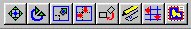
The current tool is the one currently selected (pressed
down)
 Moving tool
Click with the mouse’s left button on the selected image(s),
and drag them where you want.
 Manual rotating tool
Click with the mouse’s left button on the selected image(s)
and drag the mouse to rotate them around their center.
 Manual Scaling tool
Click with the mouse’s left button on the selected image(s)
and drag the mouse to scale them up or down around their center.
 Crop tool
Enables you to crop an image on its left, right top or bottom
side.
Click with the mouse’s left button near a border of the
selected image, and drag the mouse keeping the button down. The side that
will be cropped depends on the initial movement of the mouse. If this is vertical,
it will be the top or bottom side (whichever is nearer the cursor), and if
this is horizontal, it will be the left or right side.
The Crop tool definitively suppresses the cropped parts,
and only allows horizontal or vertical cropping. To have a more selective
cropping, refer to tool number 8 to define the navigable area.
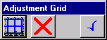
 Adjustment Tool
This is one of the most important tools of the ScanNav workshop.
It enables you to merge several scans to rebuild an entire chart.
WARNING: The image(s) on which the operations will take
place is (are) the one(s) selected when you enter this function. So Make sure to select THE and only THE piece you want to adjust!
When you select this tool, the following control box appears:
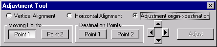
Proceed as follows:
·
Select the operation you want to perform (Vertical
or Horizontal alignment, or Adjustment of points)
·
Define all the necessary points needed for
the selected function: Select one of the « Point » buttons, and
click on the map with the mouse’s LEFT button to define the point.
·
You can move the selected point using the
arrow buttons.
·
Click on the « Adjust » button to
perform the operation
The number of points needed depend on the selected operation:
Lets you straighten up a map by aligning two points vertically
or horizontally. In this mode, you will have to define moving points 1 and
2. When you click on « Adjust », point 2 will move to align vertically
or horizontally with point 1. You can also define the « Destination »
Point 1. In this case the « Moving » point 1 will move there in
the same operation.
Adjustment Origin to destination
For this operation, you have to define all the 4 points.
When you click on « Adjust », « Moving Point 1 » will
move to « Destination Point 1 » and « Moving Point 2 »
will move to « Destination Point 2 », the selected image being transformed
in consequence. You can omit one of the « Destination » points.
In this case it will be assumed to be at the same position than it’s corresponding
« Moving » point.
You may also use this function to perform a simple translation
of the selected image. To do so, just select « Moving Point 1 »
and « Destination Point 1 » leaving both « Points 2 »
undefined.
To leave the adjustment tool, you just have to click on
the window's closing cross of the dialog box. In this case, no confirmation
is asked, and if an operation is in progress, it is aborted.
You can also leave the function by selecting another current
tool. In this case, ScanNav will ask you confirmation. This can be a way of
erasing all defined points in a row…
You also can use some keyboard shortcuts:
·
« Backspace » key: to erase the
current point.
·
1 2 3 and 4 keys: shortcut for selecting the
current point. 1 is for « Moving Point 1 », 2 for « Moving
Point 2 », 3 for « Destination Point 1 », and 4 for « Destination
Point 2 ».
·
a z q s keys: shortcut to the control box
arrows. They move the current point of one pixel towards left (a), right (z),
bottom (q), or top (s). If you leave the key down, the point will keep moving
until you release the key.
That’s for the principle. Now, you have to know that you
can zoom in and out, and move around the screen with the + and - keys, arrow
keys, or using the mouse wheel and center button. You will indeed need to
zoom in at a maximum, so as to have a maximum of precision for the definitions
of points. (You can zoom out afterwards to move around the map faster). You
can also use the zoom-in window so
as not to permanently zoom in and out.
Practical advises to use adjustment:
So as not to propagate errors while adjusting pieces, it
is recommended to proceed as follows:
·
Always start the adjustment by a central
piece of the chart, and « turn » around it. Most people have the
reflex to start from an angle, which means the adjustment errors will propagate
from one edge to the other.
·
Start adjustment by straightening up the first
scan with the vertical or horizontal alignment function. This way it
will be easier to visualize errors along the vertical or horizontal axis.
·
You can use the georeferencement grid to visualize
perfect horizontal and vertical axis on which you can align parallels and
meridians. (See hereunder for manipulation of the grid)
·
If for some reason or other you’re having
trouble to adjust a whole chart (for example if it’s too crumbled, or with
too deep folding marks…), don’t insist! In this case, instead of merging the
chart in it’s integrality, just make several blocks by merging for example
by blocks of 4 pieces, and georeferencing them separately. The blocks will
merge together in any case automatically in navigation mode, and the georeference
errors will be limited (but the frontier between blocks will me more visible
on the screen)
·
You can also retouch an adjustment after having
georeferenced the chart
Georeferencing
charts:
Once charts have been merged, you have to georeference them.
ScanNav supports different projection types (Mercator and
UTM), and takes in account the Datum specifications for the chart's referencement.
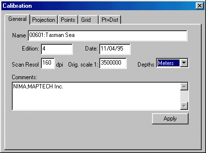
When you select this tool, the following control box shows
up.
The first tab lets you enter the chart's general parameters
The second tab lets you choose projection and datum parameters:
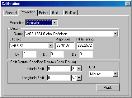
Projection
parameter:
4 types of projection are supported up to now:
1.
Latitude/Longitude projection (equidistant
Mercator projection): All the parallels are equally distant each other on
one map. This was the only projection type used by ScanNav in the first release.
This was sufficient for detailed maps, but the problem of this system is when
you start having large-scale charts where you can have a considerable difference
concerning latitude intervals at the top and the bottom of the chart. This
was resolved with tool number 7 (see next chapter), which can modify the chart
to have equidistant latitudes, but also to correct errors due to folds, etc…
It is still present for historical reasons, but should not be used anymore.
2.
Mercator Projection: It is The projection used for marine charts. This type
of projection is supported since release 1.6, so it isn't necessary to correct
latitudes with tool 7 anymore
3.
UTM Projection: This type of projection is used for topographic maps such
as the USGS DRG charts. These are not for navigation usage, but are interesting
for hikers or roadrunners, and there are sites where you can download them
for free as they are of public domain. You can also use them as a complement
to your navigation paper charts, as they also cover all the USA coasts.
4.
Lambert Projection: This projection is very much used in land cartography,
especially for the French IGN institute. There are several additional parameters
to give for the Lambert projection. These can be input through the 2 additional
fields of the dialog box that appear when the Lambert projection is selected:
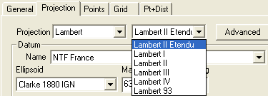
A predefined list contains the Lambert variations used by
the IGN French institute. Warning, the Datum is in close relation
with these parameters, and is not positioned automatically when choosing one
of these entries. You will therefore have to make sure you position it to
the appropriate value. Except contradictory advice on the printed map, the
Datum must be:
·
NTF France:
for « Lambert I » « Lambert II » « Lambert III »
« Lambert IV » and « Lambert II étendu »
·
WGS84: for « Lambert 93 »
The « Advanced » button lets
you define the different Lambert parameters for zones not in this list, using
the following dialog:
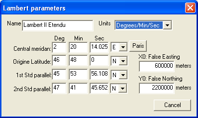
·
If you only change the name, a button « Rename »
will appear (on the left of the « Cancel » button).
·
As soon as one of the other parameters change,
a « Create » button appears instead, which lets you add entries
to the predefined list. Make sure when doing so, to also give a new name to
this entry, as there is no control on the name which can be confusing… Also
be aware that there is no way to remove entries using this interface. So limit
the different test entries to a minimum.
·
The « Paris » button lets you set
in a fast manner the Central meridian to the Paris meridian still very much
used in Lambert projection.
WARNING: A chart library must only contain maps with
the same projection parameter; otherwise adjustments between the maps will
be approximate, so erroneous. If you want to use
two charts of different projection systems in the same library, you will have
to re-project one of them using the “Reproject chart” function accessible
thru the “Operation” menu.
Datum
parameters:
The Datum specifies parameters that were used by the cartography
to reference the chart. It consists of a reference ellipsoid, and of corrections
to apply on 3 axes. A Datum name list is available, in which you can choose.
You also can enter the numeric values in the appropriate fields. The datum
is normally indicated on the chart. For recent charts it is normally the "WGS84
Global Definition". If you don't have the information on the datum, I
suggest you stick with WGS84. This datum may be specified as a name, in which
case you will have to choose in the list, but it can also be given as numeric
values. The ellipsoid is consisted of a Major Axis, and a Minor
Axis. These can be given in different forms. In general, you will
have the Major Axis and the flattening, where
flattening = (Minor Axis) / (Major Axis). Furthermore, for precision
reasons, the flattening is most often given than it's inverse
(1/flattening). This is the form in which ScanNav expects you to enter
these parameters. If you have them in another form, you might have to look
for your calculator. Then come the translation parameters Dx,
Dy, and Dz, all together forming the Datum.
Once these values entered or chosen from the list, you will
have to click on the "Apply" button so as they take effect
in ScanNav.
All this is quite complicated, and it is not so easy to
know the exact datum the original chart was calculated with. On some charts,
you will just find shift information to apply to the WGS84 reference. As an
example, on the chart number 6966 of the SHOM you will find indicated: "Positionnement
par satellites: les positions obtenus au moyen de systèmes de navigation par
satellites rapportées au système géodésique mondial WGS84 doivent être corrigées
de 0.06' vers le Nord et de 0.08' vers l'Est pour être en accord avec cette
carte", which means in English: "Satellite positioning
systems: Positions obtained with a GPS using the WGS84 datum must be moved
0.06' Northward and 0.08' Eastward to agree with this chart" . It is then simpler to just enter this shift
information, than to look for the exact datum in the list (Actually this same
chart also specifies it is in "European 1950", but this is not always
the case.)
So, a new possibility
has been added to enter the datum with these shift information’s. For the
above example, you will have to choose the WGS84
datum, and enter the following shift information:
·
Latitude shift: 0.06 N (N, as positions
given by the GPS must be moved North)
·
Longitude shift: 0.08 E (E, as positions
given by the GPS must be moved East)
This way of entering the datum is much simpler than to look
in the list, and gives good enough precision for most charts. This system
might also be applied with other datum than WGS84
Important notices:
·
Positioning errors due to a wrong datum can
vary up to several hundred meters. So it is very important that you make sure
you have chosen the right Datum when creating your own charts.
·
See also the Navigation.htm
- Datum chapter for how to set to the GPS and grid datum parameters.
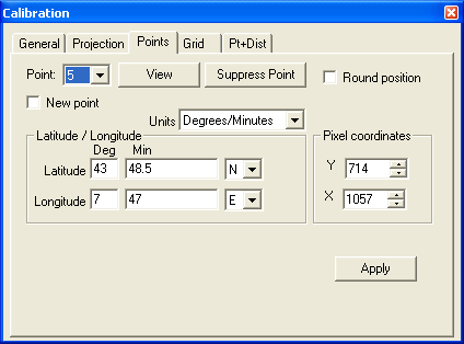
Points and reference Grid:
The following tabs are used to define the georeference grid.
In a first step, only 2 points are required. You will have to make sure those
two points are not aligned on a same latitude or longitude axis. They only
serve for elaborating a georeference grid, which you can manipulate
afterwards to fine tune the georeferencement.
Proceed as follows:
·
For more precision, use the zoom-in
window
·
Select the « Points » tab. A combo
list lets you choose the point you want to define. You have to define a minimum
of 2 points (In a first time, those two points are predefined to arbitrary
values). Select point 1 and click on a known point of the chart with the mouse’s
Left button to define the first point
·
Enter this point’s geographic position in
the appropriate fields. Values can be entered in Latitude/Longitude in “Degrees”,
“Degrees/Minutes” or “Degrees/Minutes/Seconds” for Mercator projection, or
in metric for Lambert and UTM projections.
·
Repeat the operation for the second point.
Make sure not to place this second point on the same latitude or longitude
axis.
·
Once the 2 points defined, click on the « Apply
» button to validate. The grid is then set up right, and when defining extra
points, they will be set with no correction needed if you use the “round position”
accordingly (see further).
·
In theory, 2 points are enough to reference
a chart. But certain charts might not be straight due to age, or scanner skewing.
Adding extra reference points, you can correct these imperfections. ScanNav
lets you create as many reference points as needed. To add a new point, check
the "New Point" box. Than a new point will be created each
time you click on the map.
·
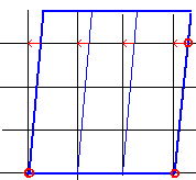
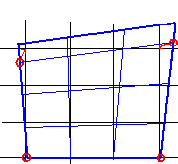
A 3rd point will let you correct
skewed charts, which is the most current deformation when scanning (where
meridians and parallels are not perpendicular). Make sure not to align the
3 points. The best is to take 3 points near the chart's opposite corners.
Using a 4th point, you can correct a second level of skew, where
meridians or parallels are no longer parallel together:
| 3
points |
4
points |
|
 |
 |
·
Other points can be added to fine tune georeference
in case of really damaged charts. In this case, you have to spread these points
regularly on the chart.
·
Adding extra points can be made very easy
using the « Round position » option.
When clicking on the chart while this
option is checked, the create/modified point is automatically rounded to the
nearest geographic position according to the input round parameters. This
greatly improves facility to add reference points by for example on crossing
of latitude and longitude lines prints in Mercator, or on the Lambert printed
cross for Lambert projection, as if the round parameter as been set appropriately
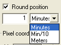
you will not have to change the position field. Make sure to choose a round
value in ad equation with the chart scale, and with the right Unit
(Minutes or Min/A0 for Mercator, Meters for UTM or Lambert). Also be aware
that in order for the rounding to work well, you will have to have done a
first calibration using 2 or 3 points as described above.
·
If you create an extra point by mistake, you
can remove it by selecting it in the list and clicking on "Suppress
point".
·
Clicking on the map without the option “new
point” checked redefines the currently selected point.
·
To move to a point's location, select it and
click "View"
You also have the possibility to work directly with the
grid, after having roughly defined two points:
·
Select the « Grid » Tab. This lets
you manipulate the created grid to fine-tune your referencement.
With this method, you don’t need to make Ultra-Precise referencement
in the first go. In fact, the two points you just created are just needed
to generate a reference grid, which you can manipulate afterwards when the
« Grid » radio button is checked.
By clicking with the mouse’s LEFT button on a meridian or
parallel line, you can drag the grid in longitude or latitude moving the line
at the position it should be, and you define the meridian or parallel that
will serve as reference for the following action (it turns red).
By clicking with the RIGHT button on a line, you move this
line to it’s new position, while the « reference » line selected
in the previous action doesn’t move, the other meridians or parallels moving
proportionally.
You can by this mean adjust the georeferencement visually
at the pixel. Nevertheless, this adjustment only stretches latitude and longitude
lines in a uniform way, and doesn’t substitute to creating additional reference
points in case of distorted charts.
The « Grid Step » button opens up a dialog that
lets you enter the desired grid spacing. (You can also use the "Grid"
entry of the "Options" menu or the « Navigation » tab
of the « preference » dialog to enter the grid spacing)
Georeference by one point and a distance:
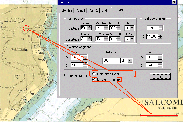
Some navigation guides contain small portions of detailed
maps representing harbor entries or other. Most of the times these maps do
not have 2 dots to calibrate, but only one dot and a scale. This georeference
method has been added and is reserved for this purpose. Make sure your Datum
is correctly set as those small maps often do not specify it, and this can
provoke a shift of several hundred meters.
This method is performed in two steps:
·
Check the "Reference point" box,
and define the known point on the screen by clicking on it. Then enter its
coordinates.
·
Check the "Distance segment" box
and define the know distance on the screen: One first click to start the segment,
and another to end it. Then enter its value in the appropriate field.
·
Then press the Apply button to validate.
Scan defaults corrections:
Warning: This functionality is obsolete.
It is still present only for historical reasons and will probably be ripped
off in future releases. It is strongly recommended not to use it anymore and
to prefer added additional reference points to correct distorted charts.
As we saw above, in its first releases,
ScanNav didn’t take in account any geodesic system to make its calculations.
These were based on an equidistant latitudes Mercator grid. But for large-scale
maps, this isn’t the case and you could have a considerable difference between
the spacing of latitudes at the top and the bottom of the map, what could
give big positioning errors. Now the true Mercator projection is supported,
but scanned charts still can be irregular, due for example to folding marks
or just to old and scrambled charts.
This tool is there to solve this problem.
It modifies the chart according to a grid that can be automatically generated
and adjusted by the user. It is nevertheless nearly obsolete, referencing
with a lot of points being more efficient. This tool should now only be used
in certain few specific cases, and will probably disappear or be adapted in
future release. This step must be performed AFTER the adjustment
and 1st step georeference. Make sure in the 1st step
reference that the extreme points (left, bottom, right, and top) of the chart
have been correctly referenced. On large-scale maps, make sure you have selected
the right projection type (Mercator). If you chose Latitude/Longitude instead,
you will see that the intermediate latitudes of the grid don’t fit the exact
latitudes. There may also be a non-fit even in longitude, due to distortions
of the scanned map. This Tool is going to help you reestablish the concordance
by defining your own grid independently of any complicated formula (you don’t
need to know the exact geodesic system of your chart, and there are no formula
that I know for distortions…) To do so, follow the different steps:
When you select tool number 7, the
following control bar appears:
 Opens the following
dialog box:
Opens the following
dialog box:
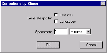
This gives you the opportunity to
generate an automatic grid in latitude and/or in longitude. You can for example
ask for a grid spacing of 1 Minute of arc, you will then just need to perfect
the georeferencement by moving each individual line of the grid to it’s right
place.
You can also define individual longitude
and/or latitude axes:
·
Double-click with the
mouse’s Left button on a known point of the map. A dialog box appears with
the actual latitude/longitude of this point. You may modify these values,
and create longitude and/or latitude axes (use the appropriate check box)
that you may manipulate later.

You may move a previously defined
axis by clicking on it with the Left button. In opposite to the 1st
step referencement, an axis moves independently to other axes.
You may also modify the latitude (or
longitude) of an axis, or suppress the axis, using the contextual menu that
appears when you click with the mouse’s right button on it.
 Once your grid defined, press on this button
to validate the action. Each individual piece of the map is going to be stretched
or compressed so the defined grid fits to a uniform grid.
Once your grid defined, press on this button
to validate the action. Each individual piece of the map is going to be stretched
or compressed so the defined grid fits to a uniform grid.
 Clicking on
this button erases the entire grid.
Clicking on
this button erases the entire grid.
Notices:
·
Dialog boxes differ
a little if the chart is in the UTM projection
·
So as not to be perturbed
by the ScanNav’s georeference grid and confuse it with your own grid, temporarily
disable it by pressing the « 0 » (zero) keyboard key, or with the
"Grid" entry of the "Options" menu, or in the « preference »
menu.
·
This functionality only
corrects the cylindrical projections like Mercator (parallels and meridians
must be perpendicular)
·
This functionality regenerates
all the images of the chart. This has the following consequences:
·
All the overlaps of
the different scans are eliminated.
·
Adjustment between the
different scans will then be not so easily retouched.
·
The operation can last
a time (a progress bar gives you indications on the advancement)
·
WARNING: for the demo version, this functionality generates
charts with the incrusted copyright notice.
My advice is to backup the chart in
a file with the original scans, before performing this step. This will enable
people who work with the demo version not to have to re-scan and merge all
their charts again, but only perform this last action, if they decide to acquire
the official release. You might also find out after a while that an adjustment
isn’t so good, and needs to be retouched.
 Definition of
the navigable area
Definition of
the navigable area
This tool lets you define the area of the chart that will be visible
in navigation mode when the option “Hide non navigable area” is checked, the
rest of the chart being hidden. This avoids to hide a useful part of a chart
with a non navigable part (such as the frame) of an adjacent chart, but still
keeping this frame for other various uses such as printing or verifying the
georeferencing.
Compared to the “Crop” tool, this tool keeps the hidden area, and lets
you define any polygonal area, whereas the “Crop” tool deletes the cropped
area, and is limited to vertical or horizontal cropping. The Crop tool is
nevertheless still useful to eliminate large Blanc areas that you’ll never
need, which saves space on disc and memory.
Defining the navigable area is quite simple. It is the same
as for the definition of the danger areas: click on the map with the mouse’s
left button on different spots to surround the area. Each click creates a
new segment. To finish the area definition, you can either double-click on
the last point, or press the keyboard “Entry” key. When clicking with the
mouse’s right button you suppress last defined point, and by pressing the
keyboard “Esc” key, you abort the area definition.
Once the area is defined, it is displayed with a bold red
contour line.
Defining the navigable must be the last step. Indeed, if
you add an image that gets out of the navigable area, the area will not grow,
so you’ll have to define it again.
When you insert a map already defining a navigable area,
the area is affected to the global chart if no other area was defined before.
But if an area was already defined, this one will not change.
The goal is to modify chart portions using an external tool to incorporate
updates, and reintegrate the changes to the original chart. This is to be
done by small portions (limited to an area of 1024x768 pixels, but smaller
areas are recommended). The ergonomics will evolve in future releases. For
now you can use the following method:
- Maintain the F6 keyboard key down, and click and
drag on the map to define the rectangular area to update (you can also alternatively
select the « export area » entry of the « function »
menu)
- When releasing the mouse button, a dialog box will appear
asking you where to save the mini-map on disk.
- A new map is then created, limited to the defined area.
A map named “test” will be constituted of the following elements:
- File test.map: this contains referencement
info of the map. Do not modify it.
- test_files directory: This will contain a file with the image of the defined
area. The format of the image should directly be readable using any image
modification tool such as Paint, Photoshop, NavCor,… It will be in bmp,
gif, or tiff, depending on the selected parameter in the “Charts Generation”
tab of the ScanNav preferences. Note: Bmp format will not be compressed
to the ScanNav format like in regular charts, so as to be readable using
standard tools. It will therefore take more disk space than regular charts
Next step is to modify the chart image using the tool of
your choice, with just making sure that you keep it the same width and
height, and then save it under the same name.
- Load the original chart in workshop mode
- Insert the modified mini-chart. It should appear at the
bottom left of the screen
- Click on the mini-chart with the mouse’s right button,
and select the “adjust to reference” entry of the menu
- è The mini-chart should then overlay its original location to patch
it.
- You can save the chart as is, or optimize it for navigation,
in which case the mini-chart will be definitively incrusted in the original
chart.
Zoom-In
window:
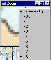
This window is activated through the "Zoom Window"
entry of the "View" menu.
It shows the main window's cursor area at the specified
zoom level. This enables you to have good precision on delicate operation
such as adjustment or georeferencement without having to zoom in and out continuously.
It isn't a pixel zoom of the main window but a real zoom of the origin image.
So the chosen zoom level is independent of the main window's zoom level.
By clicking on this window with the mouse's right button,
you get a contextual menu the lets you choose the zoom level, as well as to
force the window to stay in the foreground (always on top).
This window can also be resized at wish (by pulling on it's
frame), so that the zoomed area's size can be changed.
This window is interactive. If you click inside with the
mouse's left button, it's just as if you clicked on the corresponding pixel
(or rather the fraction of pixel) of the main window. This gives you an extreme
precision, without having to zoom in and out on the main window. As the
zoom window refreshes permanently to show the cursor region, you have to stop
this refreshing so as to be able to move inside it. So when the cursor is
inside the area you want to work on, just type on the 'z' key of your
keyboard. Then you can move to the zoom window, without it changing, work
on it by clicking inside, and when you're finished and want it to restart
refreshing, just hit the 'z' key again.
Other operations on charts:
With the « Operations » menu, you can perform
several actions on the selected images
·
Color Reduction:
Lets you reduce the number of colors of the selected images to 16 or 256 colors.
Be careful this action is not reversible (no possible Undo). This is useful
when you work with images imported at a format of 16 24 or 32 bits. It improves
display speed, decreases memory usage, and mostly permits showing the right
colors if your display is 256 colors.
·
Foreground/Background: Puts the selected images in the foreground or background.
·
Original transform:
eliminates all transformations made on the selected images (scale, rotation,
and adjustment) to show them as they are on disk.
·
Reference: defines the selected chart as the reference for calculations (the
grid, and position calculations will be based on it’s georeference)
·
Adjust to reference:
adjusts all the selected charts to fit to the reference: chart are moved and
scaled to fit to the reference. Notice: this is done automatically while in
navigation mode.
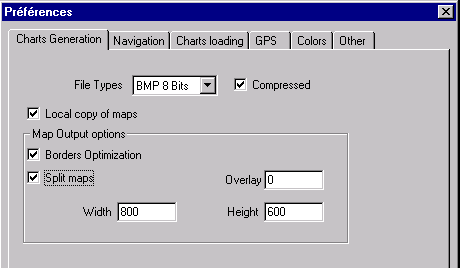
Exporting and Saving Charts:
Descriptions of ScanNav charts are stored in files with
the « .MAP » extension. They contain the chart’s reference information
as well as pointers to raster image files composing the chart. The « Charts »
tab of the « Preferences » dialog lets you parameter the raster
files characteristics:
ScanNav supports in this version 4 types of raster file
format:
·
Three standard raster formats: GIF, BMP (4
8 16 24 and 32 bits) and TIFF
·
Compressed
BMP (4 8 16 24 and 32 bits)
Images generated by ScanNav can be in any of these formats.
Nevertheless, it is strongly recommended to use the 8bits Compressed
BMP for the following reasons:
·
The 16, 24, and 32 bits BMP file formats just
increase the disk and memory usage, as well as the performances in certain
cases.
·
GIF which was the recommend format in previous
releases (compressed BMP didn’t exist) is much slower to load and takes a
bit more space on disk.
·
Standard BMP is faster to load, but takes
much more disk space
There are two ways to save a chart:
You only save the information of the « .MAP »
file (pointers to existing raster files, plus transformations to apply to
these images). Raster images will only be written on disk if:
·
They do not already exist (case of a Twain
Scan)
·
You made essential modifications on them (color
reduction, crop or grid stretching)
·
You forced ScanNav to save them anyway by
selecting the option « Local copy of maps » in « Menu-File-Preference »
tab « Maps »
The chart is cut into pieces, and overlapping pieces are
got rid of, so as to optimize memory management, loading/unloading, and drawing
times while in navigation mode, as well as disk space. In this case, raster
images are entirely re-written on disk. Since release 2.0, if the chart is
distorted (by entering more than 2 reference points) ScanNav also proposes
you to reproject the chart before saving it. Doing this enhances the speed
and automatic stitching of charts in navigation mode.
The Width and Height input fields let you enter the basic
size in pixels of each raster piece.
The Overlay parameter lets you define an overlay (in pixels)
of pieces on each other. It is of no use in ScanNav, and this value should
always be 0. It is only meant to eventually export charts to other software
that would need such an overlay.
The « borders optimization » check box should
always be checked. It enables you, when you save with « Optimize for
navigation », to save on disk only the useful parts of the chart, instead
of saving the entire rectangular bounding box which can contain blank areas.
Chart Thumbnails generation:
ScanNav can generate a thumbnail for each chart. This thumbnail
can then be shown in a small separate window that lets you move quickly around
the map. (See Using chart thumbnails
in the "Navigation" part of this manual).
This thumbnail is created automatically when you use the "Export"
function with the "Map" format, and on demand if you use the "Save"
(or "Save As"). In this case a dialog appears asking you if you
want to generate a thumbnail.
« .Map » files can be anywhere on your disk. You
must be advised that ".map" files only contain georeferencement
information and links to image files. Image files belonging to a chart will
be saved in a subdirectory having the same name as the ".map" file,
suffixed by « _Files ». As an example, raster image files belonging
to the chart « c:\charts\toto.map » will be stored in directory
« c:\charts\toto_Files\ ». Nevertheless, if you didn't check
the "Local copy of maps" check box nor used "optimize
for navigation" to save your chart, the image files can be anywhere
on disk at their original place.
So to copy a chart (on CD-ROM for example), you have to
make sure to:
·
Have checked "Local copy of maps"
when saving your chart, or saved it with "optimize for navigation".
·
Copy the ".map" file as well as
the associated "_Files" directory and its included files.
Exporting standard raster images
of the chart:
You can also save an entire chart as a raster image in GIF,
TIFF or BMP format with the « Export » menu. This way, you can use
them in any imaging software, or even other navigation aid software (let’s
stay open!). This way, you can use ScanNav for other purposes such as scanning
posters, etc...
Printing
of charts:
Printing is accessible trough the "File" menu.
You can either directly print or use the "Print Preview" to visualize
on screen the layout of different pages. In both cases the options dialog
is the same:
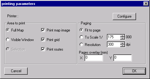
Printer used, as well as it's parameters (Portrait/landscape,
paper format, etc…) can be chosen with the button "Configure" that
opens a standard Windows dialog.
You can choose to print the entire chart, or just the visible
window. Be Careful if you choose "Full map", this represents the
full working area of ScanNav, that means all the charts loaded at that
moment. This can thus generate an impressing amount of data with which
your printer, (and even your PC) will have trouble dealing with, and you'll
get an unreadable result if you chose "Fit to Page", or empty out
you paper tray if you chose a multi-pages mosaic. So it is recommended that
you do this operation in Workshop mode, being sure you only have one map loaded.
The "selection" choice is grayed out, as not implemented in this
release.
You can choose one or more topics to print among:
·
The map image.
·
The ScanNav grid: Its step will be the one
configured at that moment.
·
Routes: This in fact includes all referenced
objects: routes, waypoints, tracks and danger areas.
Paging comports several options:
·
Fit to page: In this case, the printed topics
will be scaled to fit in one page.
In the 2 other cases, printing will
be made on a mosaic of several pages.
·
To scale 1/XX: here you give the printing
scale you want.
·
Resolution XXX: Warning, this is not the printing
resolution, but the image resolution. If you give the same value as the original
scan's resolution, you'll get an output at the same scale as the original
paper chart. If you give a higher value the resulting output will be smaller,
and if you give a smaller value, it will be larger.
For these last 2 options, you can choose an overlap between
pages. This is given in millimeters.
Printing problems: Certain print drivers can cause dysfunction
in ScanNav, and certain work better than others can. Some crashes have been
reported when printing, mostly with postscript printers under Windows 95/98
(Windows NT has much less problems). So it is important to save your work
before you print anything. In case of a crash or a dysfunction try the
following manipulations:
·
Optimize the chart for navigation: this generates
more homogeneous images lighter to mange for the printer.
·
Try another driver for the printer: as an
example Postscript printers can often be managed in PCL5 mode, and a printer
can often be driven by a driver of another similar printer.
·
Try to suppress elements to print (for example
the grid, or just change it's step…).
·
Please report me your dysfunction problems
with the more information you can.
In the Demo version, any image generated by ScanNav will
be incrusted with a copyright label inside.
Top of page
 Georeferencement Tool
 Grid tool